MCMC Algorithm for BART-STAR — bart

Run the MCMC algorithm for a BART model for count-valued responses using STAR. The transformation can be known (e.g., log or sqrt) or unknown (Box-Cox or estimated nonparametrically) for greater flexibility.

Usage

bart_star(
  y,
  X,
  X_test = NULL,
  y_test = NULL,
  transformation = "np",
  y_max = Inf,
  n.trees = 200,
  sigest = NULL,
  sigdf = 3,
  sigquant = 0.9,
  k = 2,
  power = 2,
  base = 0.95,
  nsave = 1000,
  nburn = 1000,
  nskip = 0,
  save_y_hat = FALSE,
  verbose = TRUE
)

Arguments

y

n x 1 vector of observed counts

X

n x p matrix of predictors

X_test

n0 x p matrix of predictors for test data

y_test

n0 x 1 vector of the test data responses (used for computing log-predictive scores)

transformation

transformation to use for the latent process; must be one of

"identity" (identity transformation)
"log" (log transformation)
"sqrt" (square root transformation)
"np" (nonparametric transformation estimated from empirical CDF)
"pois" (transformation for moment-matched marginal Poisson CDF)
"neg-bin" (transformation for moment-matched marginal Negative Binomial CDF)
"box-cox" (box-cox transformation with learned parameter)
"ispline" (transformation is modeled as unknown, monotone function using I-splines)

y_max

a fixed and known upper bound for all observations; default is Inf

n.trees

number of trees to use in BART; default is 200

sigest

positive numeric estimate of the residual standard deviation (see ?bart)

sigdf

degrees of freedom for error variance prior (see ?bart)

sigquant

quantile of the error variance prior that the rough estimate (sigest) is placed at. The closer the quantile is to 1, the more aggressive the fit will be (see ?bart)

k

the number of prior standard deviations E(Y|x) = f(x) is away from +/- 0.5. The response is internally scaled to range from -0.5 to 0.5. The bigger k is, the more conservative the fitting will be (see ?bart)

power

power parameter for tree prior (see ?bart)

base

base parameter for tree prior (see ?bart)

nsave

number of MCMC iterations to save

nburn

number of MCMC iterations to discard

nskip

number of MCMC iterations to skip between saving iterations, i.e., save every (nskip + 1)th draw

save_y_hat

logical; if TRUE, compute and save the posterior draws of the expected counts, E(y), which may be slow to compute

verbose

logical; if TRUE, print time remaining

Value

a list with the following elements:

post.pred: draws from the posterior predictive distribution of y
post.sigma: draws from the posterior distribution of sigma
post.log.like.point: draws of the log-likelihood for each of the n observations
WAIC: Widely-Applicable/Watanabe-Akaike Information Criterion
p_waic: Effective number of parameters based on WAIC
post.pred.test: draws from the posterior predictive distribution at the test points X_test (NULL if X_test is not given)
post.fitted.values.test: posterior draws of the conditional mean at the test points X_test (NULL if X_test is not given)
post.mu.test: draws of the conditional mean of z_star at the test points X_test (NULL if X_test is not given)
post.log.pred.test: draws of the log-predictive distribution for each of the n0 test cases (NULL if X_test is not given)
fitted.values: the posterior mean of the conditional expectation of the counts y (NULL if save_y_hat=FALSE)
post.fitted.values: posterior draws of the conditional mean of the counts y (NULL if save_y_hat=FALSE)

In the case of transformation="ispline", the list also contains

post.g: draws from the posterior distribution of the transformation g
post.sigma.gamma: draws from the posterior distribution of sigma.gamma, the prior standard deviation of the transformation g() coefficients

If transformation="box-cox", then the list also contains

post.lambda: draws from the posterior distribution of lambda

Details

STAR defines a count-valued probability model by (1) specifying a Gaussian model for continuous *latent* data and (2) connecting the latent data to the observed data via a *transformation and rounding* operation. Here, the model in (1) is a Bayesian additive regression tree (BART) model.

Posterior and predictive inference is obtained via a Gibbs sampler that combines (i) a latent data augmentation step (like in probit regression) and (ii) an existing sampler for a continuous data model.

There are several options for the transformation. First, the transformation can belong to the *Box-Cox* family, which includes the known transformations 'identity', 'log', and 'sqrt', as well as a version in which the Box-Cox parameter is inferred within the MCMC sampler ('box-cox'). Second, the transformation can be estimated (before model fitting) using the empirical distribution of the data y. Options in this case include the empirical cumulative distribution function (CDF), which is fully nonparametric ('np'), or the parametric alternatives based on Poisson ('pois') or Negative-Binomial ('neg-bin') distributions. For the parametric distributions, the parameters of the distribution are estimated using moments (means and variances) of y. Third, the transformation can be modeled as an unknown, monotone function using I-splines ('ispline'). The Robust Adaptive Metropolis (RAM) sampler is used for drawing the parameter of the transformation function.

Examples

# \donttest{
# Simulate data with count-valued response y:
sim_dat = simulate_nb_friedman(n = 100, p = 5)
y = sim_dat$y; X = sim_dat$X

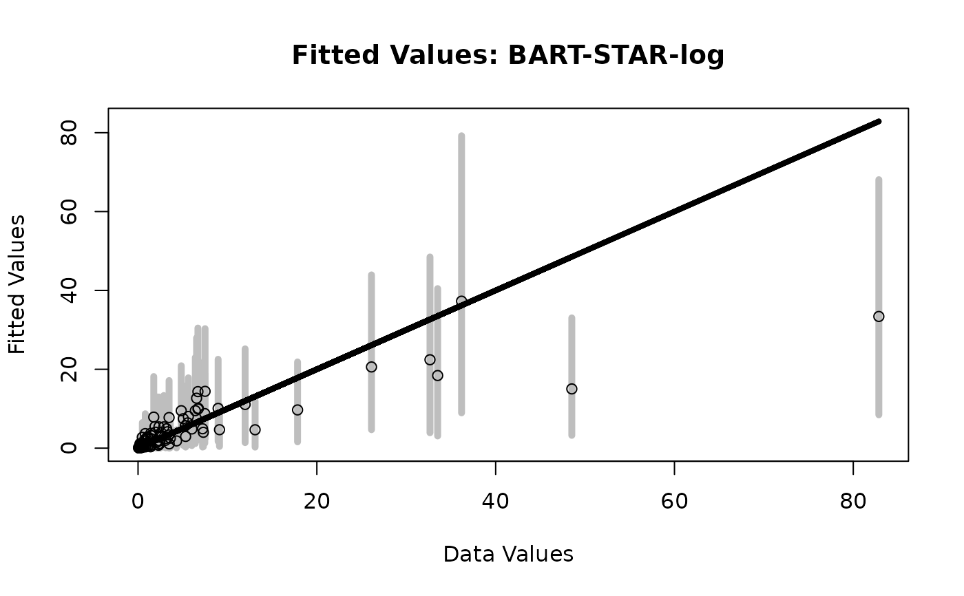
# BART-STAR with log-transformation:
fit_log = bart_star(y = y, X = X, transformation = 'log',
                    save_y_hat = TRUE, nburn=1000, nskip=0)
#> [1] "Burn-In Period"
#> [1] "Starting sampling"
#> [1] "0 seconds remaining"
#> [1] "Total time:  2 seconds"

# Fitted values
plot_fitted(y = sim_dat$Ey,
            post_y = fit_log$post.fitted.values,
            main = 'Fitted Values: BART-STAR-log')


# WAIC for BART-STAR-log:
fit_log$WAIC
#> [1] 382.4023

# MCMC diagnostics:
plot(as.ts(fit_log$post.fitted.values[,1:10]))


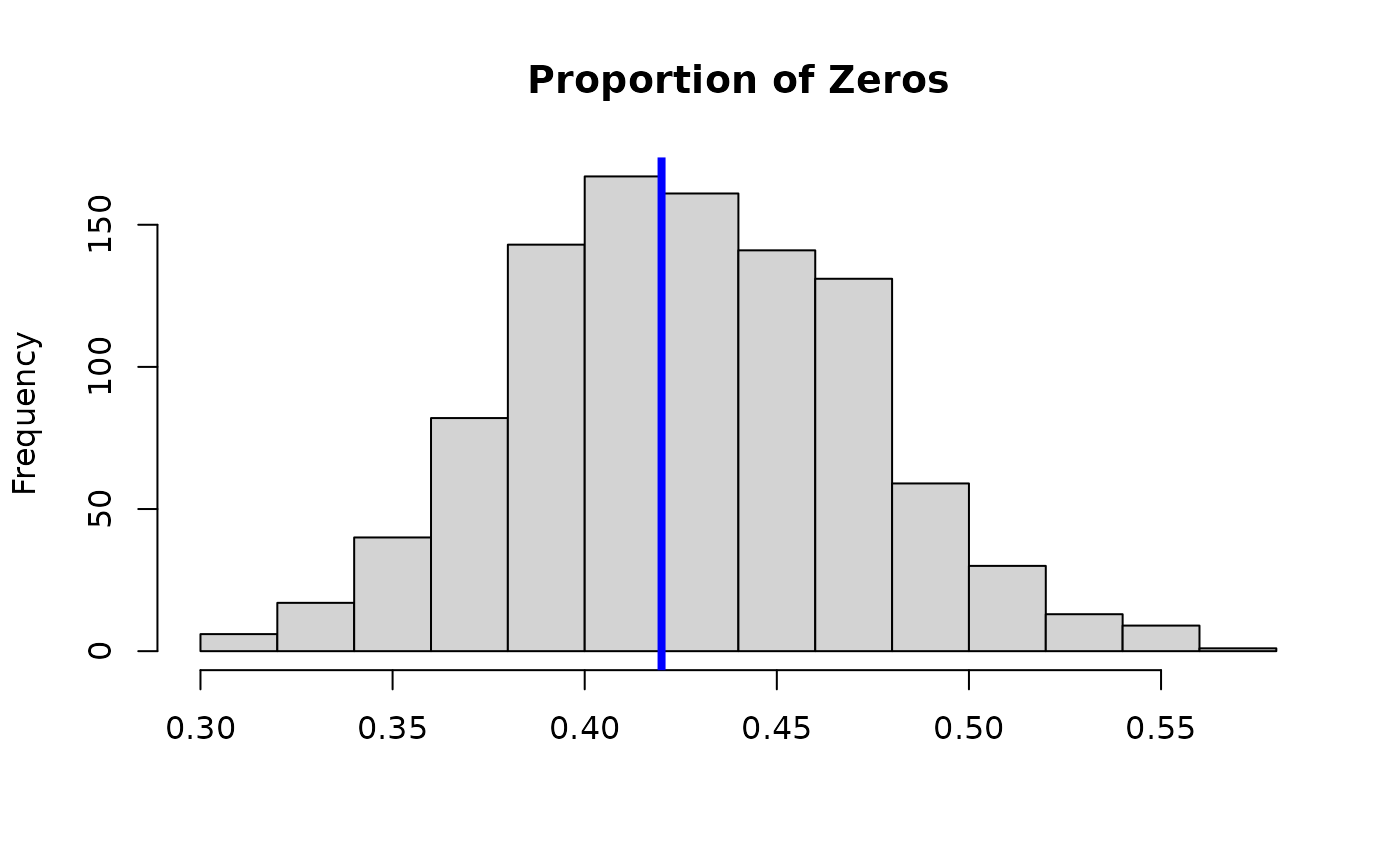
# Posterior predictive check:
hist(apply(fit_log$post.pred, 1,
           function(x) mean(x==0)), main = 'Proportion of Zeros', xlab='');
abline(v = mean(y==0), lwd=4, col ='blue')


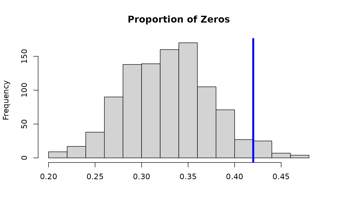
# BART-STAR with nonparametric transformation:
fit = bart_star(y = y, X = X,
                     transformation = 'np', save_y_hat = TRUE)
#> [1] "Burn-In Period"
#> [1] "Starting sampling"
#> [1] "0 seconds remaining"
#> [1] "Total time:  4 seconds"

# Fitted values
plot_fitted(y = sim_dat$Ey,
            post_y = fit$post.fitted.values,
            main = 'Fitted Values: BART-STAR-np')


# WAIC for BART-STAR-np:
fit$WAIC
#> [1] 379.1259

# MCMC diagnostics:
plot(as.ts(fit$post.fitted.values[,1:10]))


# Posterior predictive check:
hist(apply(fit$post.pred, 1,
           function(x) mean(x==0)), main = 'Proportion of Zeros', xlab='');
abline(v = mean(y==0), lwd=4, col ='blue')

# }