Getting Started with countSTAR

Introduction

The countSTAR package implements a variety of methods to analyze count data, all based on Simultaneous Transformation and Rounding (STAR) models. The package functionality is broadly split into three categories: frequentist/classical estimation (Kowal and Wu (2021)), Bayesian modeling and prediction (Kowal and Canale (2020); Kowal and Wu (2022)), and time series analysis and forecasting (King and Kowal (2023)).

We give a brief description of the STAR framework, before diving into specific examples that show the countSTAR functionality.

STAR Model Overview

STAR models build upon continuous data models to provide a valid count-valued data-generating process. As a motivating example, consider the common practice of taking log- or square-root transformations of count data and then applying continuous data models (e.g., Gaussian or OLS regressions). This approach is widely popular because it addresses the skewness often found in count data and enables use of familiar models, but it does not provide a valid count data distribution. STAR models retain the core components—the transformation and the continuous data model—but add in a rounding layer to ensure a coherent, count-valued data-generating process. For example: $$\begin{align*} y_i &= \mbox{floor}(y_i^*) \\ z_i &= \log(y_i^*) \\ z_i &= x_i'\theta + \epsilon_i, \quad \epsilon_i \sim N(0, \sigma^2) \end{align*}$$ The transformation and continuous data model are not applied directly to the observed counts $y_i$, but rather to a latent “continuous proxy” $y_i^*$. The (latent) continuous data model is linked to the (observed) count data via a coarsening operation. This is not the same as rounding the outputs from a fitted continuous data model: the discrete nature of the data is built into the model itself, and thus is central in estimation, inference, and prediction.

More generally, STAR models are defined via a rounding operator $h$, a (known or unknown) transformation $g$, and a continuous data model with unknown parameters $\theta$: $$\begin{align*} y_i &= h(y_i^*) \quad \mbox{(rounding)}\\ z_i &= g(y_i^*) \quad \mbox{(transformation)}\\ z_i &= \mu_\theta(x_i) + \epsilon_i \quad \mbox{(model)}\\ \end{align*}$$ usually with $\epsilon_i \sim N(0, \sigma^2)$. Examples of $\mu_\theta(x)$ include linear, additive, and tree-based regression models. The regression model may be replaced with a time series model (see warpDLM(), discussed below) or other continuous data models.

STAR models are highly flexible models and provide the capability to model count (or rounded) data with challenging features such as

• zero-inflation
• over- or under-dispersion
• bounded or censored data
• heaping or multi-modality

all with minimal user inputs and within a regression (or time series) context.

The Rounding Operator

The rounding operator $h$ is a many-to-one function (or coarsening) that sets $y = j$ whenever $y^*\in A_j$ or equivalently when $z \in g(A_j)$. The floor function $A_j := [j, j+1)$ works well as a default, with modifications for lower and upper endpoints. First, $g(A_0) := (-\infty, 0)$ ensures that $y = 0$ whenever $z < 0$. Much of the latent space is mapped to zero, which enables STAR models to account for zero-inflation. Similarly, when there is a known (finite) upper bound y_max for the data, we fix $g(A_K) := [g(a_K), \infty)$, so STAR models can capture endpoint inflation. In fact, because of the coarsening nature of STAR models, they equivalently can be applied for count data that are bounded or censored at y_max without any modifications (Kowal and Canale (2020)). From the user’s perspective, only y_max needs to be specified (if finite).

The Transformation Function

There are a variety of options for the transformation function $g$, ranging from fixed functions to data-driven estimates to fully Bayesian (nonparametric) models for the transformation.

First, all models in countSTAR support three fixed transformations: log, sqrt, and identity (essentially a rounding-only model). In these cases, the STAR model has exactly the same number of unknown parameters as the (latent) continuous data model. Thus, it gives a parsimonious adaptation of continuous data models to the count data setting.

Second, most functions support a set of transformations that are estimated by matching marginal moments of the data $y$ to the latent $z$:

• transformation='np' is a nonparametric transformation estimated from the empirical CDF of $y$
• transformation='pois' uses a moment-matched marginal Poisson CDF
• transformation='neg-bin' uses a moment-matched marginal Negative Binomial CDF.

Details on the estimation of these transformations can be found in Kowal and Wu (2021). The nonparametric transformation np is effective across a variety of empirical examples, so it is the default for frequentist STAR methods. The main drawback of this group of transformations is that, after being estimated, they are treated as fixed and known for estimation and inference of $\theta$. Of course, this drawback is limited when $n$ is large.

Finally, Bayesian STAR methods enable joint learning of the transformation $g$ along with the model parameters $\theta$. Thus, uncertainty about the transformation is incorporated into all downstream estimation, inference, and prediction. These include both nonparametric and parametric transformations:

• transformation='bnp': the transformation is modeled using Bayesian nonparametrics, and specifically via a Dirichlet process for the marginal outcome distribution, which incorporates uncertainty about the transformation into posterior and predictive inference.
• transformation='box-cox': the transformation is assumed to belong to the Box-Cox family; the $\lambda$ parameter can be fixed or learned.
• transformation='ispline': the transformation is modeled as an unknown, monotone function using I-splines. The Robust Adaptive Metropolis (RAM) sampler is used for the unknown transformation $g$.

The transformation bnp is the default for all applicable Bayesian models. It is nonparametric, which provides substantial distributional flexible for STAR regression, and is remarkably computationally efficient—even compared to parametric alternatives. This approach is inspired by Kowal and Wu (2025).

For any countSTAR function, the user can see which transformations are supported by checking the appropriate help page, e.g., ?blm_star().

Count-Valued Data: The Roaches Dataset

As an example of challenging count-valued data, consider the roaches data from Gelman and Hill (2006). The response variable, $y_i$, is the number of roaches caught in traps in apartment $i$, with $i=1,\ldots, n = 262$.

data(roaches, package="countSTAR") 

# Roaches:
y = roaches$y

# Plot the PMF:
plot(0:max(y), 
     sapply(0:max(y), function(js) mean(js == y)), 
     type='h', lwd=2, main = 'PMF: Roaches Data',
     xlab = 'Roaches', ylab = 'Probability mass')

There are several notable features in the data:

1. Zero-inflation: 36% of the observations are zeros.
2. (Right-) Skewness, which is clear from the histogram and common for (zero-inflated) count data.
3. Overdispersion: the sample mean is 26 and the sample variance is 2585.

A pest management treatment was applied to a subset of 158 apartments, with the remaining 104 apartments receiving a control. Additional data are available on the pre-treatment number of roaches, whether the apartment building is restricted to elderly residents, and the number of days for which the traps were exposed. We are interested in modeling how the roach incidence varies with these predictors.

# Design matrix:
X = model.matrix( ~ roach1 + treatment + senior + log(exposure2),
                 data = roaches)

head(X)
#>   (Intercept) roach1 treatment senior log(exposure2)
#> 1           1 308.00         1      0     -0.2231436
#> 2           1 331.25         1      0     -0.5108256
#> 3           1   1.67         1      0      0.0000000
#> 4           1   3.00         1      0      0.0000000
#> 5           1   2.00         1      0      0.1335314
#> 6           1   0.00         1      0      0.0000000

Frequentist inference for STAR models

Frequentist (or classical) estimation and inference for STAR models is provided by an EM algorithm. Sufficient for estimation is an estimator function which solves the least squares (or Gaussian maximum likelihood) problem associated with $\mu_\theta$—or in other words, the estimator that would be used for Gaussian or continuous data. Specifically, estimator inputs data and outputs a list with two elements: the estimated coefficients $\hat \theta$ and the fitted.values $\hat \mu_\theta(x_i) = \mu_{\hat \theta}(x_i)$. countSTAR includes implementations for linear, random forest, and generalized boosting regression models (see below), but it is straightforward to incorporate other models via the generic genEM_star() function.

The STAR Linear Model

For many cases, the STAR linear model is the first method to try: it combines a rounding operator $h$, a transformation $g$, and the latent linear regression model $$\begin{align*} z_i &= x_i'\theta + \epsilon_i, \quad \epsilon_i \sim N(0, \sigma^2) \end{align*}$$ In countSTAR, the (frequentist) STAR linear model is implemented with lm_star() (see blm_star() for a Bayesian version). lm_star() aims to mimic the functionality of lm by allowing users to input a formula. Standard functions like coef and fitted can be used on the output to extract coefficients and fitted values, respectively.

library(countSTAR)

# EM algorithm for STAR linear regression
fit = lm_star(y ~ roach1 + treatment + senior + log(exposure2),
              data = roaches, 
              transformation = 'np')

# Fitted coefficients:
round(coef(fit), 3)
#>    (Intercept)         roach1      treatment         senior log(exposure2) 
#>          0.035          0.006         -0.285         -0.321          0.216

Here the frequentist nonparametric transformation was used, but other options are available; see ?lm_star() for details.

Based on the fitted STAR linear model, we may further obtain confidence intervals for the estimated coefficients using confint():

# Confidence interval for all coefficients
confint(fit)
#>                       2.5 %       97.5 %
#> (Intercept)    -0.139711518  0.199942615
#> roach1          0.004898573  0.007468304
#> treatment      -0.488199761 -0.085641963
#> senior         -0.548729134 -0.102510551
#> log(exposure2) -0.197843036  0.636935236

Similarly, p-values are available using likelihood ratio tests, which can be applied for individual coefficients,

$$H_0: \theta_j= 0 \quad \mbox{vs.} \quad H_1: \theta_j \ne 0$$

or for joint sets of variables, analogous to a (partial) F-test:

$$H_0: \theta_1=\ldots=\theta_p = 0 \quad \mbox{vs.} \quad H_1: \theta_j \ne 0 \mbox{ for some } j=1,\ldots,p$$ P-values for all individual coefficients as well as the p-value for any effects are computed with the pvals() function.

# P-values:
round(pvals(fit), 4)
#>        (Intercept)             roach1          treatment             senior 
#>             0.6973             0.0000             0.0056             0.0049 
#>     log(exposure2) Any linear effects 
#>             0.3072             0.0000

Finally, we can get predictions at new data points (or the training data) using predict().

#Compute the predictive draws (just using observed points here)
y_pred = predict(fit)

For predictive distributions, blm_star() and other Bayesian models are recommended.

STAR Machine Learning Models

countSTAR also includes STAR versions of machine learning models: random forests (randomForest_star()) and generalized boosted machines (gbm_star()). These refer to the specification of the latent regression function $\mu_\theta(x)$ along with the accompanying estimation algorithm for continuous data. Here, the user directly inputs the set of predictors $X$ alongside any test points in $X_{test}$, excluding the intercept:

#Fit STAR with random forests
suppressMessages(library(randomForest))
fit_rf = randomForest_star(y = y, X = X[,-1], # no intercept 
                           transformation = 'np')

#Fit STAR with GBM
suppressMessages(library(gbm))
fit_gbm = gbm_star(y = y, X = X[,-1], # no intercept 
                   transformation = 'np')

For all frequentist models, the functions output log-likelihood values at the MLEs, which allows for a quick comparison of model fit.

#Look at -2*log-likelihood
-2*c(fit_rf$logLik, fit_gbm$logLik)
#> [1] 1666.783 1593.495

In general, it is preferable to compare these fits using out-of-sample predictive performance. Point predictions are available via the named components fitted.values or fitted.values.test for in-sample predictions at $X$ or out-of-sample predictions at $X_{test}$, respectively.

Bayesian inference for STAR models

Bayesian STAR models only require an algorithm for (initializing and) sampling from the posterior distribution under a continuous data model. In particular, the most convenient strategy for posterior inference with STAR is to use a data-augmentation Gibbs sampler, which combines that continuous data model sampler with a draw from the latent data posterior, $[z | y, \theta]$, which is a truncated (Gaussian) distribution. For special cases of Bayesian STAR models, direct Monte Carlo (not MCMC) sampling is available.

Efficient algorithms are implemented for several popular Bayesian regression and time series models (see below). The user may also adapt their own continuous data models and algorithms to the count data setting via the generic function genMCMC_star().

Bayesian STAR Linear Model

Revisiting the STAR linear model, the Bayesian version places a prior on $\theta$. The default in countSTAR is Zellner’s g-prior, which has the most functionality, but other options are available (namely, horseshoe and ridge priors). The model is estimated using blm_star(). Note that for the Bayesian models in countSTAR, the user must supply the design matrix $X$ (and if predictions are desired, a matrix of predictors at the test points). We apply this to the roaches data, now using the default Bayesian nonparametric transformation:

fit_blm = blm_star(y = y, X = X, 
                   transformation = 'bnp')

In some cases, direct Monte Carlo (not MCMC) sampling can be performed (see Kowal and Wu (2022) for details): simply set use_MCMC=FALSE. Although it is appealing to avoid MCMC, the output is typically similar and the Monte Carlo sampler requires truncated multivariate normal draws, which become slow for large $n$.

Posterior expectations and posterior credible intervals from the model are available as follows:

# Posterior mean of each coefficient:
round(coef(fit_blm),3)
#>    (Intercept)         roach1      treatment         senior log(exposure2) 
#>          0.316          0.008         -0.388         -0.420          0.284

# Credible intervals for regression coefficients
ci_all_bayes = apply(fit_blm$post.beta,
      2, function(x) quantile(x, c(.025, .975)))

# Rename and print:
rownames(ci_all_bayes) = c('Lower', 'Upper')
print(t(round(ci_all_bayes, 3)))
#>                 Lower  Upper
#> (Intercept)     0.020  0.605
#> roach1          0.006  0.010
#> treatment      -0.648 -0.122
#> senior         -0.717 -0.127
#> log(exposure2) -0.220  0.831

We can check standard MCMC diagnostics:

# MCMC diagnostics for posterior draws of the regression coefficients (excluding intercept)
plot(as.ts(fit_blm$post.beta[,-1]), 
     main = 'Trace plots', cex.lab = .75)

# (Summary of) effective sample sizes (excluding intercept)
suppressMessages(library(coda))
getEffSize(fit_blm$post.beta[,-1])
#>    Min. 1st Qu.  Median    Mean 3rd Qu.    Max. 
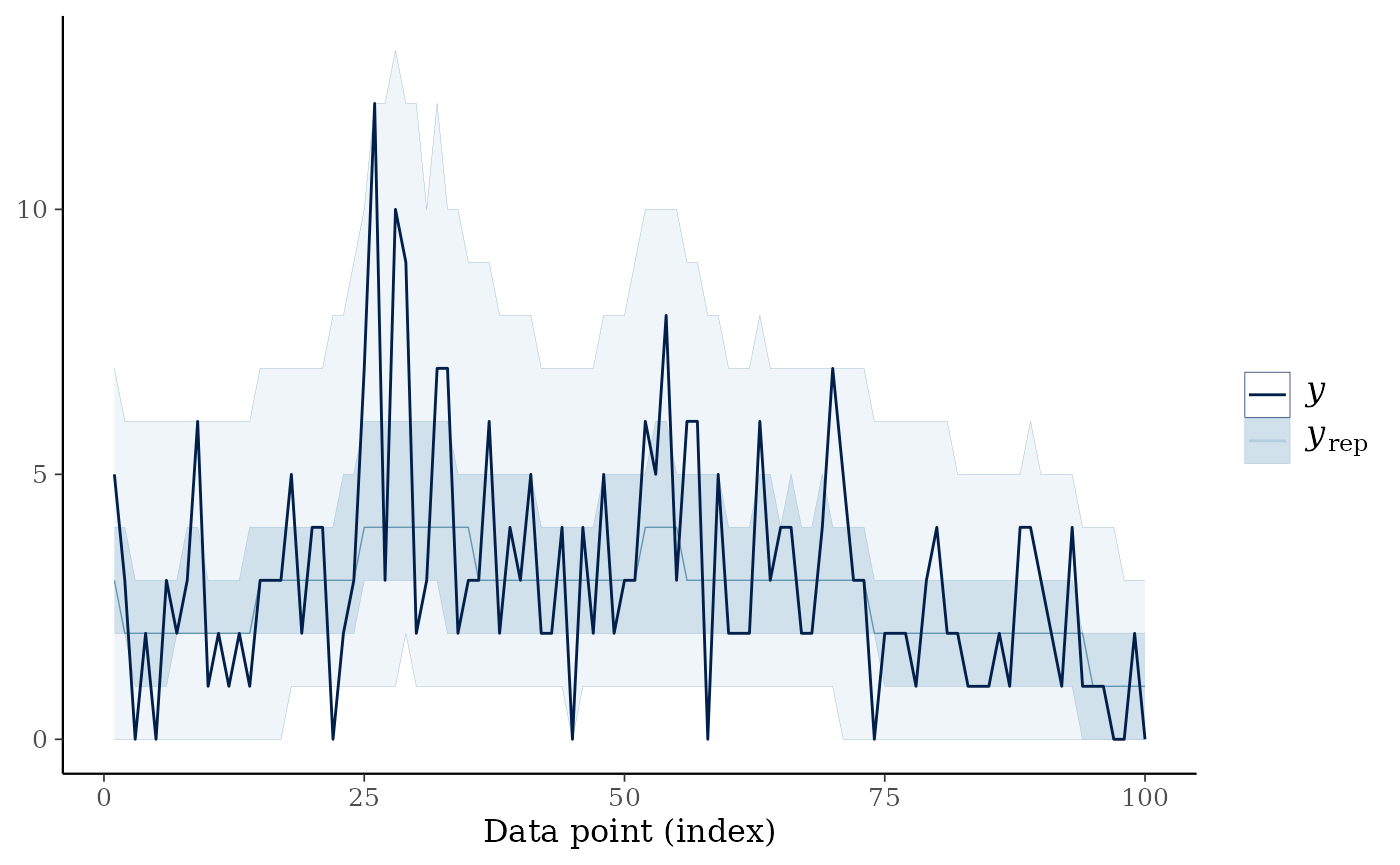
#>   676.2   736.1   759.6   798.8   822.3  1000.0

We may further evaluate the model based on posterior diagnostics and posterior predictive checks on the simulated versus observed proportion of zeros. Posterior predictive checks are easily visualized using the bayesplot package.

# Posterior predictive check using bayesplot
suppressMessages(library(bayesplot))
prop_zero = function(y) mean(y == 0)
ppc_stat(y = y, 
          yrep = fit_blm$post.pred, 
          stat = "prop_zero")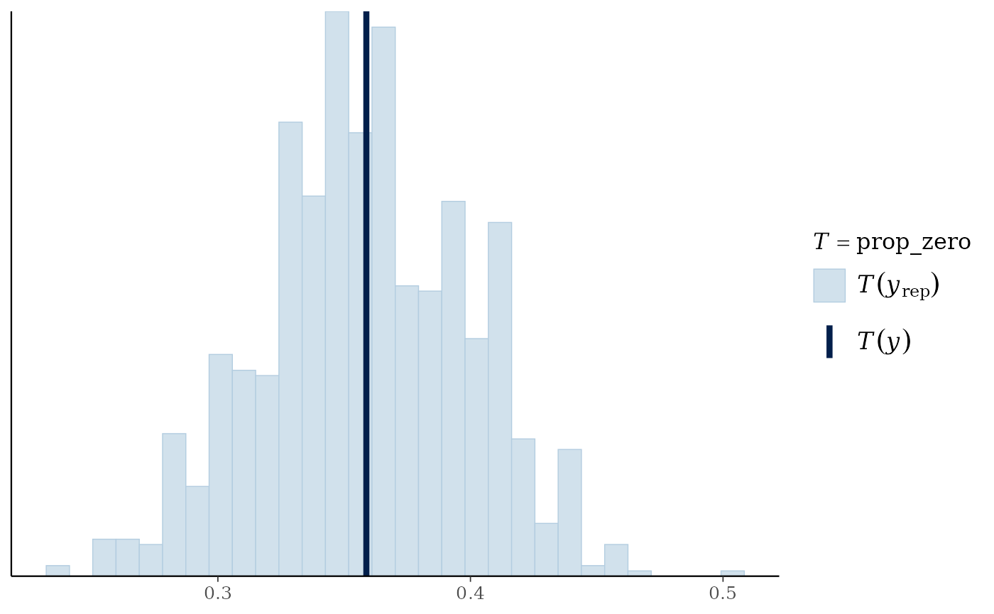

BART STAR

One of the most flexible model options is to use Bayesian Additive Regression Trees (BART; Chipman, George, and McCulloch (2012)) as the latent regression model. Here, $\mu_\theta(x)$ is a sum of many shallow trees with small (absolute) terminal node values. BART-STAR enables application of BART models and algorithms for count data, thus combining the regression flexibility of BART with the (marginal) distributional flexibility of STAR:

fit_bart = bart_star(y = y, X = X, 
                     transformation = 'np')
#> [1] "1 sec remaining"
#> [1] "Total time: 2 seconds"

Since bnp is not yet implemented for bart_star(), we use np here. The transformation is still estimated nonparametrically, but then is treated as fixed and known (see 'ispline' for a fully Bayesian and nonparametric version, albeit slower).

Once again, we can perform posterior predictive checks. This time we plot the densities:

ppc_dens_overlay(y = y, 
                 yrep = fit_bart$post.pred[1:50,])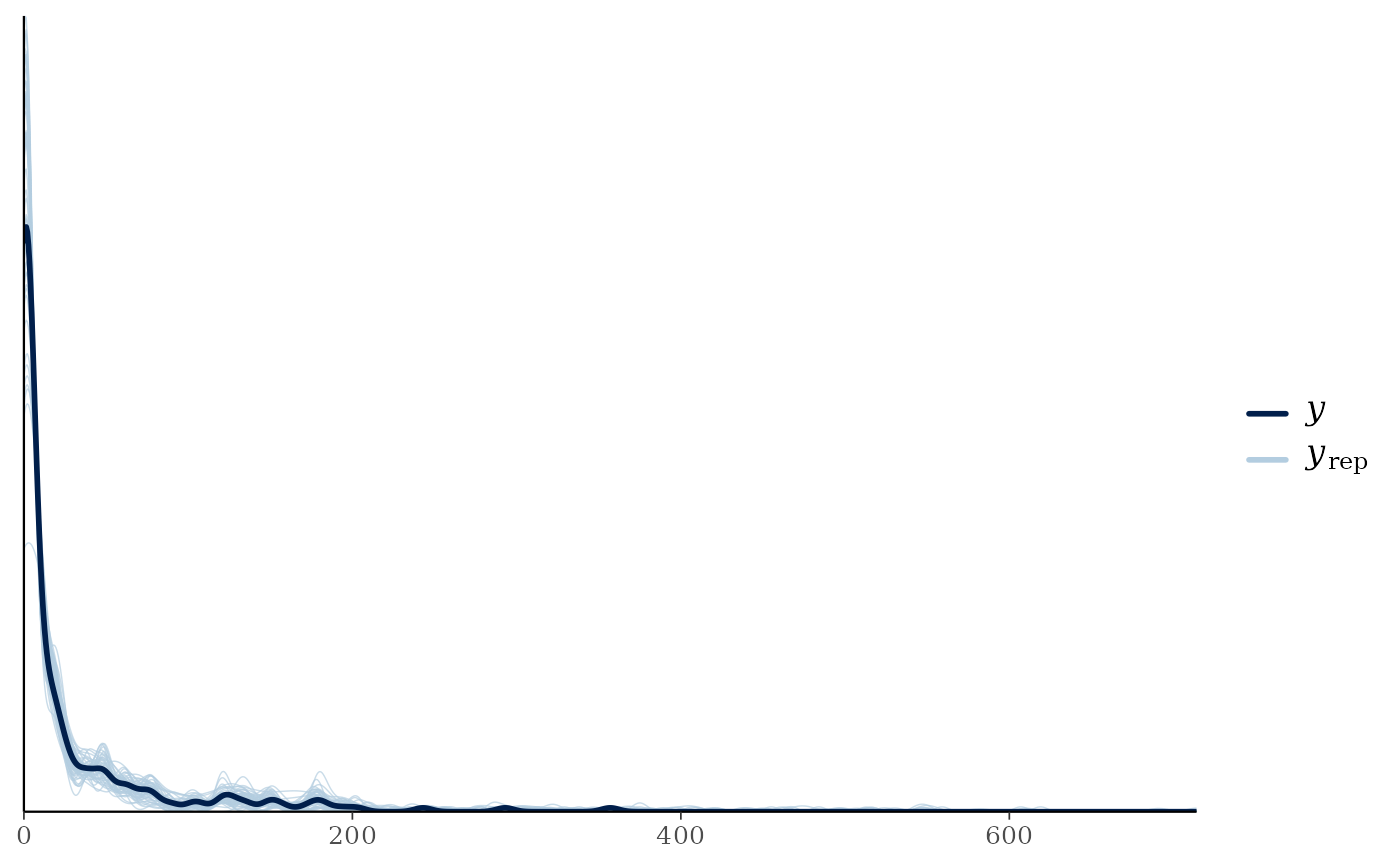

Pointwise log-likelihoods and WAIC values are outputted for model comparison. Using this information, we can see the BART STAR model seems to have a better fit than the linear model:

waic <- c(fit_blm$WAIC, fit_bart$WAIC)
names(waic) <- c("STAR Linear Model", "BART-STAR")
print(waic)
#> STAR Linear Model         BART-STAR 
#>          1762.281          1639.514

Other Bayesian Models

To estimate a nonlinear relationship between a (univariate) covariate $x$ and count-valued $y$, spline_star() implements a highly efficient, fully Bayesian spline regression model.

For multiple nonlinear effects, bam_star() implements a Bayesian additive model with STAR. The user specifies which covariates should be modeled linearly and which should be modeled nonlinearly via splines. Note that bam_star() can be slower than blm_star() or bart_star().

Count Time Series Modeling: warpDLM

Up to this point, we have focused on static regression where the data does not depend on time. Notably, King and Kowal (2023) extended STAR to the time series setting by incorporating a powerful time series framework known as Dynamic Linear Models (DLMs). A DLM is defined by two equations: (i) the observation equation, which specifies how the observations are related to the latent state vector and (ii) the state evolution equation, which describes how the states are updated in a Markovian fashion. More concretely, and using $t$ subscripts for time: $$\begin{align*} z_t &= F_t \theta_t + v_t, \quad v_t \sim N_n(0, V_t) \\ \theta_t &= G_t \theta_{t-1} + w_t, \quad w_t \sim N_p( 0, W_t) \end{align*}$$ for $t=1,\ldots, T$, where $\{ v_t, w_t\}_{t=1}^T$ are mutually independent and $\theta_0 \sim N_p(a_0, R_0)$.

Of course, given the Gaussian assumptions of the model, a DLM alone is not appropriate for count data. Thus, a warping operation—combining the transformation and rounding—is merged with the DLM, resulting in a warped DLM (warpDLM): $$\begin{align*} y_t &= h \circ g^{-1}(z_t) \\ \{z_t\}_{t=1}^T &\sim \text{DLM} \end{align*}$$

The DLM form shown earlier is very general. Among these DLMs, countSTAR currently implements the local level model and the local linear trend model. A local level model (also known as a random walk with noise model) has a univariate state $\theta_t:=\mu_t$ with $$\begin{align*} z_t &= \mu_t + v_t, \quad v_t \sim N(0, V) \\ \mu_t &= \mu_{t-1} + w_t, \quad w_t \sim N(0, W) \end{align*}$$ The local linear trend model extends the local level model by incorporating a time varying drift $\nu_t$ in the dynamics: $$\begin{align*} z_t &= \mu_t + v_t, \quad v_t \sim N(0, V) \\ \mu_t &= \mu_{t-1} + \nu_{t-1} + w_{\mu,t}, \quad w_{\mu,t} \sim N( 0, W_ \mu) \\ \nu_t &= \nu_{t-1} + w_{\nu,t}, \quad w_{\nu,t} \sim N( 0, W_\nu) \end{align*}$$ This can in turn be recast into the general two-equation DLM form. Namely, if we let $\theta_t:=(\mu_t, \nu_t)$, the local linear trend is written as $$\begin{align*} z_t & = \begin{pmatrix} 1 & 0 \end{pmatrix} \begin{pmatrix} \mu_t \\ \nu_t \end{pmatrix} + v_t, \quad v_t \sim N(0, V) \\ \begin{pmatrix} \mu_t \\ \nu_t \end{pmatrix} & = \begin{bmatrix} 1 & 1 \\ 0 & 1 \end{bmatrix} \begin{pmatrix} \mu_{t-1} \\ \nu_{t-1} \end{pmatrix} + \boldsymbol{w_t}, \quad \boldsymbol{w_t} \sim N\begin{pmatrix} \boldsymbol{0}, \begin{bmatrix} W_ \mu & 0 \\ 0 & W_\nu \end{bmatrix} \end{pmatrix} \end{align*}$$

These two common forms have a long history and are also referred to as structural time series models (implemented in base R via StructTS()). With countSTAR, warpDLM time series modeling is accomplished via the warpDLM() function. In the below, we apply the model to a time series dataset included in base R concerning yearly numbers of important discoveries from 1860 to 1959 (?discoveries for more information).

#Visualize the data
plot(discoveries)

# Required package:
library(KFAS)
#> Please cite KFAS in publications by using: 
#> 
#>   Jouni Helske (2017). KFAS: Exponential Family State Space Models in R. Journal of Statistical Software, 78(10), 1-39. doi:10.18637/jss.v078.i10.

#Fit the model
warpfit = warpDLM(y = discoveries, type = "trend")
#> [1] "Time taken:  31.846  seconds"

Once again, we can check fit using posterior predictive checks. The median of the posterior predictive draws can act as a sort of count-valued smoother of the time series.

ppc_ribbon(y = as.vector(discoveries), 
           yrep = warpfit$post_pred)

References

Chipman, Hugh A., Edward I. George, and Robert E. McCulloch. 2012. “BART: Bayesian additive regression trees.” Annals of Applied Statistics 6 (1): 266–98. https://doi.org/10.1214/09-AOAS285.

Gelman, Andrew, and Jennifer Hill. 2006. Data Analysis Using Regression and Multilevel/Hierarchical Models. Cambridge University Press.

King, Brian, and Daniel R. Kowal. 2023. “Warped Dynamic Linear Models for Time Series of Counts.” Bayesian Analysis, 1–26. https://doi.org/10.1214/23-BA1394.

Kowal, Daniel R., and Antonio Canale. 2020. “Simultaneous Transformation and Rounding (STAR) Models for Integer-Valued Data.” Electronic Journal of Statistics 14 (1). https://doi.org/10.1214/20-ejs1707.

Kowal, Daniel R., and Bohan Wu. 2021. “Semiparametric Count Data Regression for Self-Reported Mental Health.” Biometrics. https://onlinelibrary.wiley.com/doi/10.1111/biom.13617.

———. 2022. “Semiparametric Discrete Data Regression with Monte Carlo Inference and Prediction.” https://arxiv.org/abs/2110.12316.

———. 2025. “Monte Carlo Inference for Semiparametric Bayesian Regression.” Journal of the American Statistical Association 120 (550): 1063–76. https://doi.org/10.1080/01621459.2024.2395586.