Estimation for Bayesian STAR spline regression

Compute samples from the predictive distributions of a STAR spline regression model using either a Gibbs sampling approach or exact Monte Carlo sampling (default is Gibbs sampling which scales better for large n).

Usage

spline_star(
  y,
  tau = NULL,
  transformation = "np",
  y_max = Inf,
  psi = NULL,
  nsave = 1000,
  use_MCMC = TRUE,
  nburn = 1000,
  nskip = 0,
  verbose = TRUE
)

Arguments

y

n x 1 vector of observed counts

tau

n x 1 vector of observation points; if NULL, assume equally-spaced on [0,1]

transformation

transformation to use for the latent data; must be one of

• "identity" (identity transformation)

• "log" (log transformation)

• "sqrt" (square root transformation)

• "bnp" (Bayesian nonparametric transformation using the Bayesian bootstrap)

• "np" (nonparametric transformation estimated from empirical CDF)

• "pois" (transformation for moment-matched marginal Poisson CDF)

• "neg-bin" (transformation for moment-matched marginal Negative Binomial CDF)

y_max

a fixed and known upper bound for all observations; default is Inf

psi

prior variance (1/smoothing parameter); if NULL, update in MCMC

nsave

number of MCMC iterations to save (or number of Monte Carlo simulations)

use_MCMC

logical; whether to run Gibbs sampler or Monte Carlo (default is TRUE)

nburn

number of MCMC iterations to discard

nskip

number of MCMC iterations to skip between saving iterations, i.e., save every (nskip + 1)th draw

verbose

logical; if TRUE, print time remaining

Value

a list with the following elements:

• post.pred: nsave x n samples from the posterior predictive distribution at the observation points tau

• marg_like: the marginal likelihood (only if use_MCMC=FALSE; otherwise NULL)

Details

STAR defines a count-valued probability model by (1) specifying a Gaussian model for continuous *latent* data and (2) connecting the latent data to the observed data via a *transformation and rounding* operation. Here, the continuous latent data model is a spline regression.

There are several options for the transformation. First, the transformation can belong to the *Box-Cox* family, which includes the known transformations 'identity', 'log', and 'sqrt'. Second, the transformation can be estimated (before model fitting) using the empirical distribution of the data y. Options in this case include the empirical cumulative distribution function (CDF), which is fully nonparametric ('np'), or the parametric alternatives based on Poisson ('pois') or Negative-Binomial ('neg-bin') distributions. For the parametric distributions, the parameters of the distribution are estimated using moments (means and variances) of y. The distribution-based transformations approximately preserve the mean and variance of the count data y on the latent data scale, which lends interpretability to the model parameters. Lastly, the transformation can be modeled using the Bayesian bootstrap ('bnp'), which is a Bayesian nonparametric model and incorporates the uncertainty about the transformation into posterior and predictive inference.

Note

For the 'bnp' transformation there are numerical stability issues when psi is modeled as unknown. In this case, it is better to fix psi at some positive number.

Examples

# Simulate some data:
n = 100
tau = seq(0,1, length.out = n)
y = round_floor(exp(1 + rnorm(n)/4 + poly(tau, 4)%*%rnorm(n=4, sd = 4:1)))

# Sample from the predictive distribution of a STAR spline model:
fit = spline_star(y = y, tau = tau)
#> [1] "Burn-In Period"
#> [1] "Starting sampling"
#> [1] "0 seconds remaining"
#> [1] "Total time:  1 seconds"

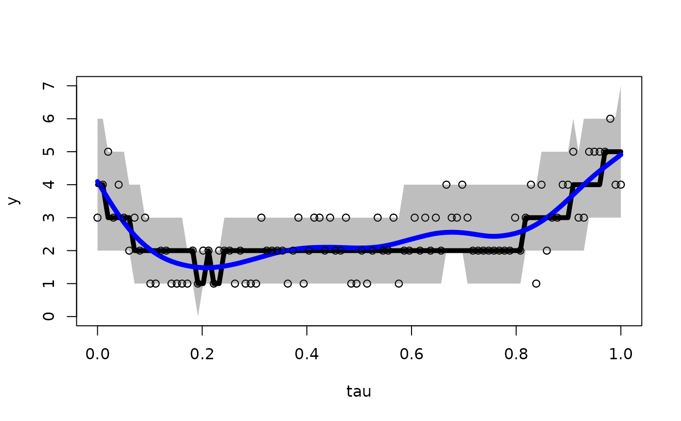
# Compute 90% prediction intervals:
pi_y = t(apply(fit$post.pred, 2, quantile, c(0.05, .95)))

# Plot the results: intervals, median, and smoothed mean
plot(tau, y, ylim = range(pi_y, y))
polygon(c(tau, rev(tau)),c(pi_y[,2], rev(pi_y[,1])),col='gray', border=NA)
lines(tau, apply(fit$post.pred, 2, median), lwd=5, col ='black')
lines(tau, smooth.spline(tau, apply(fit$post.pred, 2, mean))$y, lwd=5, col='blue')
lines(tau, y, type='p')