Posterior and predictive inference for STAR linear model
Usage
blm_star(
  y,
  X,
  X_test = X,
  transformation = "bnp",
  y_max = Inf,
  prior = "gprior",
  use_MCMC = TRUE,
  nsave = 1000,
  nburn = 1000,
  nskip = 0,
  psi = length(y),
  alpha = 1,
  F0 = NULL,
  compute_marg = FALSE,
  verbose = FALSE
)
Arguments
- y
n x 1vector of observed counts- X
n x pmatrix of predictors- X_test
n_test x pmatrix of predictors for test data; default is the observed covariatesX- transformation
transformation to use for the latent process; must be one of
"identity" (identity transformation)
"log" (log transformation)
"sqrt" (square root transformation)
"np" (nonparametric transformation estimated from empirical CDF)
"pois" (transformation for moment-matched marginal Poisson CDF)
"neg-bin" (transformation for moment-matched marginal Negative Binomial CDF)
"box-cox" (box-cox transformation with learned parameter)
"ispline" (transformation is modeled as unknown, monotone function using I-splines)
"bnp" (Bayesian nonparametric transformation)
- y_max
a fixed and known upper bound for all observations; default is
Inf- prior
prior to use for the latent linear regression; currently implemented options are "gprior", "horseshoe", and "ridge"
- use_MCMC
logical; whether to run Gibbs sampler or Monte Carlo (default is TRUE)
- nsave
number of MC(MC) iterations to save
- nburn
number of MCMC iterations to discard
- nskip
number of MCMC iterations to skip between saving iterations, i.e., save every (nskip + 1)th draw
- psi
prior variance (g-prior)
- alpha
prior precision for the Dirichlet Process prior ('bnp' transformation only); default is one
- F0
function to evaluate the base measure CDF supported on
{0,...,y_max}('bnp' transformation only)- compute_marg
logical; if TRUE, compute and return the marginal likelihood (only available when using exact sampler, i.e. use_MCMC=FALSE)
- verbose
logical; if TRUE, print time remaining
Value
a list with at least the following elements:
coefficients: the posterior mean of the regression coefficientspost.beta: posterior draws of the regression coefficientspost.pred: draws from the posterior predictive distribution ofypost.log.like.point: draws of the log-likelihood for each of thenobservationsWAIC: Widely-Applicable/Watanabe-Akaike Information Criterionp_waic: Effective number of parameters based on WAIC
Other elements may be present depending on the choice of prior, transformation, and sampling approach.
Details
STAR defines a count-valued probability model by (1) specifying a Gaussian model for continuous *latent* data and (2) connecting the latent data to the observed data via a *transformation and rounding* operation. Here, the continuous latent data model is a linear regression.
There are several options for the transformation. First, the transformation can belong to the *Box-Cox* family, which includes the known transformations 'identity', 'log', and 'sqrt', as well as a version in which the Box-Cox parameter is inferred within the MCMC sampler ('box-cox').
Second, the transformation can be estimated (before model fitting) using the
the data y. Options in this case include the empirical cumulative
distribution function (ECDF), which is fully nonparametric ('np'), or the parametric
alternatives based on Poisson ('pois') or Negative-Binomial ('neg-bin')
distributions. For the parametric distributions, the parameters of the distribution
are estimated using moments (means and variances) of y.
Lastly, the transformation can be modeled nonparametrically using (monotone) splines ('ispline') or Bayesian nonparametrics via Dirichlet processes ('bnp'). The 'bnp' option is the default because it is highly flexible, accounts for uncertainty when the transformation is unknown, and is computationally efficient.
The Monte Carlo sampler (use_MCMC=FALSE) produces direct, joint draws
from the posterior predictive distribution under a g-prior. When n is
moderate to large, or to use other priors, MCMC sampling (use_MCMC=TRUE)
is much faster and more convenient.
Examples
# \donttest{
# Simulate data with count-valued response y:
sim_dat = simulate_nb_lm(n = 100, p = 5)
y = sim_dat$y; X = sim_dat$X
# Fit the Bayesian STAR linear model:
fit = blm_star(y = y, X = X)
#> [1] "1 sec remaining"
#> Warning: Some predicted y-values growing too large! Capping to ensure algorithm completion...
#> [1] "Total time: 1 seconds"
# What is included:
names(fit)
#> [1] "coefficients" "post.beta" "post.pred"
#> [4] "post.g" "post.log.like.point" "WAIC"
#> [7] "p_waic"
# Posterior mean of each coefficient:
coef(fit)
#> [1] 0.63890524 0.42451156 0.58820069 -0.13267476 -0.09229361
# WAIC:
fit$WAIC
#> [1] 337.2181
# MCMC diagnostics:
plot(as.ts(fit$post.beta))
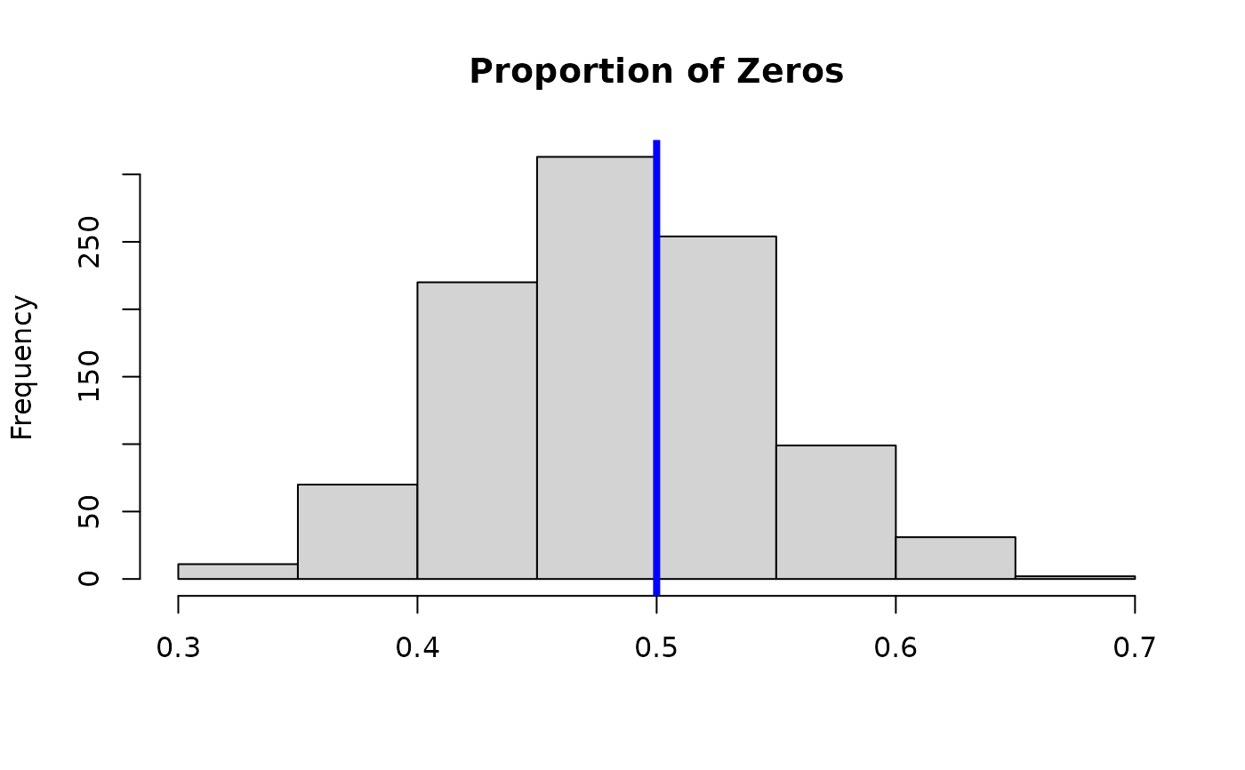
 # Posterior predictive check:
hist(apply(fit$post.pred, 1,
function(x) mean(x==0)), main = 'Proportion of Zeros', xlab='');
abline(v = mean(y==0), lwd=4, col ='blue')
# Posterior predictive check:
hist(apply(fit$post.pred, 1,
function(x) mean(x==0)), main = 'Proportion of Zeros', xlab='');
abline(v = mean(y==0), lwd=4, col ='blue')
 # }
# }