Generalized MCMC Algorithm for STAR — genMCMC

Run the MCMC algorithm for STAR given

a function to initialize model parameters; and
a function to sample (i.e., update) model parameters.

The transformation can be known (e.g., log or sqrt) or unknown (Box-Cox or estimated nonparametrically) for greater flexibility.

Usage

genMCMC_star(
  y,
  sample_params,
  init_params,
  transformation = "np",
  y_max = Inf,
  nsave = 1000,
  nburn = 1000,
  nskip = 0,
  save_y_hat = FALSE,
  verbose = TRUE
)

Arguments

y

n x 1 vector of observed counts

sample_params

a function that inputs data y and a named list params containing

mu: the n x 1 vector of conditional means (fitted values)
sigma: the conditional standard deviation
coefficients: a named list of parameters that determine mu

and outputs an updated list params of samples from the full conditional posterior distribution of coefficients and sigma (and updates mu)

init_params

an initializing function that inputs data y and initializes the named list params of mu, sigma, and coefficients

transformation

transformation to use for the latent data; must be one of

"identity" (identity transformation)
"log" (log transformation)
"sqrt" (square root transformation)
"np" (nonparametric transformation estimated from empirical CDF)
"pois" (transformation for moment-matched marginal Poisson CDF)
"neg-bin" (transformation for moment-matched marginal Negative Binomial CDF)
"box-cox" (box-cox transformation with learned parameter)

y_max

a fixed and known upper bound for all observations; default is Inf

nsave

number of MCMC iterations to save

nburn

number of MCMC iterations to discard

nskip

number of MCMC iterations to skip between saving iterations, i.e., save every (nskip + 1)th draw

save_y_hat

logical; if TRUE, compute and save the posterior draws of the expected counts, E(y), which may be slow to compute

verbose

logical; if TRUE, print time remaining

Value

a list with at least the following elements:

post.pred: draws from the posterior predictive distribution of y
post.sigma: draws from the posterior distribution of sigma
post.log.like.point: draws of the log-likelihood for each of the n observations
WAIC: Widely-Applicable/Watanabe-Akaike Information Criterion
p_waic: Effective number of parameters based on WAIC
post.lambda: draws from the posterior distribution of lambda (NULL unless transformation='box-cox')
fitted.values: the posterior mean of the conditional expectation of the counts y (NULL if save_y_hat=FALSE)
post.fitted.values: posterior draws of the conditional mean of the counts y (NULL if save_y_hat=FALSE)

If the coefficients list from init_params and sample_params contains a named element beta, e.g. for linear regression, then the function output contains

coefficients: the posterior mean of the beta coefficients
post.beta: draws from the posterior distribution of beta
post.othercoefs: draws from the posterior distribution of any other sampled coefficients, e.g. variance terms

If no beta exists in the parameter coefficients, then the output list just contains

coefficients: the posterior mean of all coefficients
post.beta: draws from the posterior distribution of all coefficients

Additionally, if init_params and sample_params have output mu_test, then the sampler will output post.predtest, which contains draws from the posterior predictive distribution at test points.

Details

STAR defines a count-valued probability model by (1) specifying a Gaussian model for continuous *latent* data and (2) connecting the latent data to the observed data via a *transformation and rounding* operation.

Posterior and predictive inference is obtained via a Gibbs sampler that combines (i) a latent data augmentation step (like in probit regression) and (ii) an existing sampler for a continuous data model.

There are several options for the transformation. First, the transformation can belong to the *Box-Cox* family, which includes the known transformations 'identity', 'log', and 'sqrt', as well as a version in which the Box-Cox parameter is inferred within the MCMC sampler ('box-cox'). Second, the transformation can be estimated (before model fitting) using the empirical distribution of the data y. Options in this case include the empirical cumulative distribution function (CDF), which is fully nonparametric ('np'), or the parametric alternatives based on Poisson ('pois') or Negative-Binomial ('neg-bin') distributions. For the parametric distributions, the parameters of the distribution are estimated using moments (means and variances) of y.

Examples

# Simulate data with count-valued response y:
sim_dat = simulate_nb_lm(n = 100, p = 5)
y = sim_dat$y; X = sim_dat$X

# STAR: log-transformation:
fit_log = genMCMC_star(y = y,
                         sample_params = function(y, params) sample_lm_gprior(y, X, params),
                         init_params = function(y) init_lm_gprior(y, X),
                         transformation = 'log')
#> [1] "Burn-In Period"
#> [1] "Starting sampling"
#> [1] "0 seconds remaining"
#> [1] "Total time:  0 seconds"

# What is included:
names(fit_log)
#>  [1] "coefficients"        "post.beta"           "post.othercoefs"    
#>  [4] "post.pred"           "post.predtest"       "post.sigma"         
#>  [7] "post.log.like.point" "WAIC"                "p_waic"             
#> [10] "post.lambda"         "fitted.values"       "post.fitted.values" 

# Posterior mean of each coefficient:
coef(fit_log)
#>        beta1        beta2        beta3        beta4        beta5 
#>  0.240239425  0.623564718  0.588955162 -0.029877031 -0.002942044 

# WAIC for STAR-log:
fit_log$WAIC
#> [1] 377.8431

# MCMC diagnostics:
plot(as.ts(fit_log$post.beta[,1:3]))


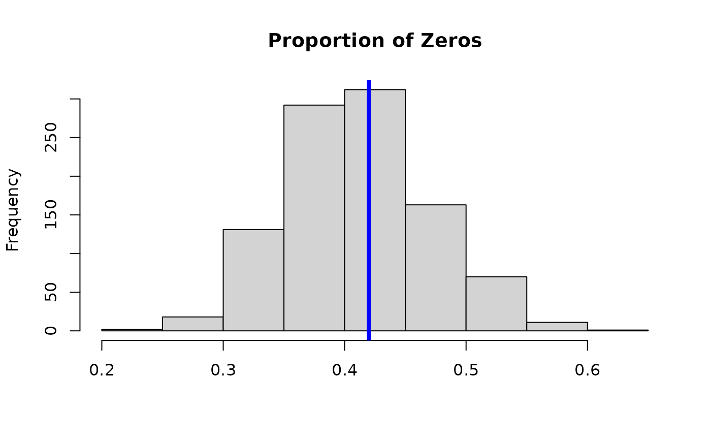
# Posterior predictive check:
hist(apply(fit_log$post.pred, 1,
           function(x) mean(x==0)), main = 'Proportion of Zeros', xlab='');
abline(v = mean(y==0), lwd=4, col ='blue')